Lesson 13

Hypothesis Testing with the t-test Statistic

Outline

Unknown Population Values

The t-distribution

-t-table

Confidence Intervals

Unknown Population Values

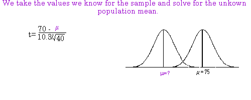
When we are testing a hypothesis we usually don’t know parameters from the population.  That is, we don’t know the mean and standard deviation of an entire population most of the time.  So, the t-test is exactly like the z-test computationally, but instead of using the standard deviation from the population we use the standard deviation from the sample. The formula is: , where   

The standard deviation from the sample (S), when used to estimate a population in this way, is computed differently than the standard deviation from the population.  Recall that the sample standard deviation is “S” and is computed with n-1 in the denominator (see prior lesson).  Most of the time you will be given this value, but in the homework packet there are problems where you must compute it yourself.

The t-distribution

There are several conceptual differences when the statistic uses the standard deviation from the sample instead of the population.  When we use the sample to estimate the population it will be much smaller than the population.  Because of this fact the distribution will not be as regular or “normal” in shape.  It will tend to be flatter and more spread out than population distribution, and so are not as “normal” in shape as a larger set of values would yield.  In fact, the t-distribution is a family of distributions (like the z-distribution), that vary as a function of sample size.  The larger the sample size the more normal in shape the distribution will be.  Thus, the critical value that cuts off 5% of the distribution will be different than on the z-score.  Since the distribution is more spread out, a higher value on the scale will be needed to cut off just 5% of the distribution.

The practical results of doing a t-test is that 1) there is a difference in the formula notation, and 2) the critical values will vary depending on the size of the sample we are using.  Thus, all the steps you have already learned stay the same, but when you see that the problem gives the standard deviation from the sample (S) instead of the population (σ), you write the formula with “t” instead of “z”, and you use a different table to find the critical value.

The t-table

Critical values for the t-test will vary depending on the sample size we are using, and as usual whether it is one-tail or two-tail, and due to the alpha level.  These critical values are in the Appendices in the back of your book.  See page A27 in your text.  Notice that we have one and two-tail columns at the top and degrees of freedom (df) down the side.  Degrees of freedom are a way of accounting for the sample size.  For this test df = n – 1.

Cross index the correct column with the degrees of freedom you compute.  Note that this is a table of critical values rather than a table of areas like the z-table.

Also note, that as n approaches infinity, the t-distribution approaches the z-distribution.  If you look at the bottom row (at the infinity symbol) you will see all the critical values for the z-test we learned on the last exam.

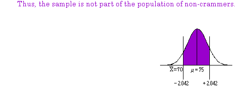
Whenever we reject the null hypothesis we are saying that the sample we are dealing with does not
come from the same population as the one we for which we know the parameters (μ ). If the distance
between the sample mean and the population mean is great enough, we must conclude that the sample
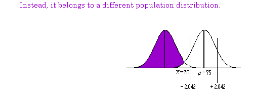
mean is part of some other population. This other population has its own set of parameters (i.e. its own
mean and standard deviation). The sample mean we have is a sample from this other population that
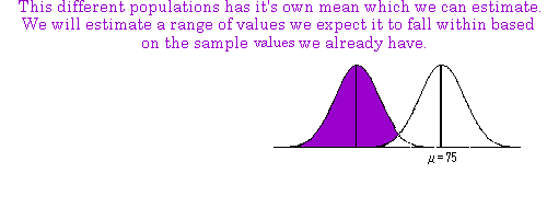
we don’t know the parameters for yet. Recall, however, that a sample mean is going to be our best
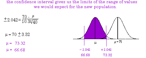
estimate of the population mean. When we calculate a confidence interval, we are using the sample
mean to estimate the parameters of this new population.
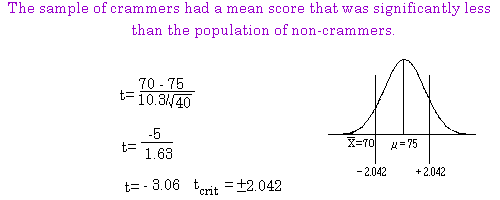
In the following example we reject the null hypothesis that students who cram for an exam score as well
as students that do not cram. The sample mean for the crammers was 70 with a standard deviation of
10.3. The sample size was N=40. We rejected the null hypothesis that this sample of crammers did as
well on an exam as non‐crammers who had a population mean of 75 (Alpha=.05; two‐tail). In the
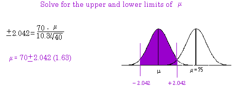
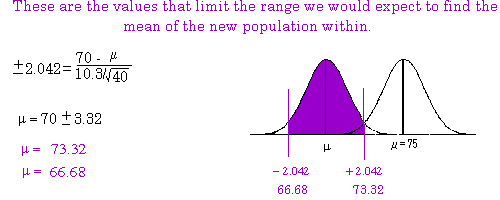
example we demonstrate how to calculate the 95% confidence interval. We will be 95% sure that the
mean of the new population (from which the sample comes) falls within the range we calculate. (Note
that the critical value should be 2.101 for our t‐table instead of 2.042 used in the example).