Lesson 15
ANOVA (analysis of variance)
Outline
Variability
-between group variability
-within group variability
-total variability
-F-ratio
Computation
-sums of squares (between/within/total)
-degrees of freedom (between/within/total)
-mean square (between/within)
-F (ratio of between to within)
Example Problem
Note: The formulas detailed here vary a great deal from the text. I suggest using the notation I have outlined here since it will coincide more with what we have already done, but you might look at the text version as well. Use whatever method you find easiest to understand.
Variability
You can read background information about this topic on the web page by locating the ANOVA demonstration or you can click here: http://faculty.uncfsu.edu/dwallace/sanova.html
Between group variability and within group variability are both components of the total variability in the combined distributions. What we are doing when we compute between and within variability is to partition the total variability into the between and within components. So: Between variability + within variability = total variability
Hypothesis Testing
Again, with ANOVA we are testing hypotheses that involve comparisons of two or more populations. The overall test, however, will indicate a difference between any of the groups. Thus, the test will not specify which two, or if some or all of the groups differ. Instead, we will conduct a separate test to determine which specific means differ. Because of this fact the research hypothesis will state simply that “at least two of the means differ.” The null will still state that there are no significant differences between any of the groups (insert as many “mu’s” as you have groups). H0: m1=m2=m3
Critical values are found using the F-table in your book. The table is discussed in the example below.
Computation
How do we measure variability in a distribution? That is, how do we measure how different scores are in the distribution from one another? You should know that we use variance as a measure of variability. With ANOVA or analysis of variance, we compute a ratio of variances: between to within variance. Recall that variance is the average square deviation of scores about the mean. We will compute the same value here, but as the definition suggests, it will be called the “mean square” for the computations.
So, we are computing variance. Recall that when we compute variance we first find the sum of the square deviations, and then divide by the sample size (n -1 or degrees of freedom for a sample).
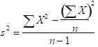
When we compute the Mean Square (variance) in order to form the F-ratio, we will do the exact same thing: compute the sums of squares and divide by degrees of freedom. Don’t let the formulas intimidate you. Keep in mind that all we are doing is finding the variance for our between factor and dividing that by the variance for the within factor. These two variances will be computing by finding each sums of squares and dividing those sums of squares by their respective degrees of freedom.
Sums of Squares
We will use the same basic formula for sums of squares that we used with variance. While we will only use the between variance and within variance to compute the F-ration, we will still compute the sums of squares total (all values) for completeness.
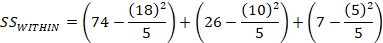
Total Sums of Squares
Note that it is the same formula we have been using. The subscript (tot) stands for the total. It indicates that you perform the operation for ALL values in your distribution (all subjects in all groups).
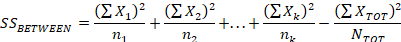
Within Sums of Squares

Notice that each segment is the same formula for sums of squares we used in the formula for variance and for the total sums of squares above. What is different here is that you consider each group separately. So, the first segment with the subscript “1” means you compute the sum of squares for the first group. Group two is labeled with a “2”, but notice that after that we have group “k” instead of a number. This notation indicates that you continue to find the sums of squares as you did for the first two groups for however many groups you have in the problem. So, “k” could be the third group, or if you have four groups then you would do the same sums of squares computation for the third and fourth group.
Between Sums of Squares
We have the same “k” notation here. Again, you perform the same operation for each separate group in your problem. However, with this formula once we compute the value for each group we must subtract an operation at the final step. This operation is half the sums of squares we computed for the sums of squares total.
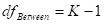
Degrees of Freedom
Again, we will first compute the sums of squares for each source of variance, divide the values by degrees of freedom in order to get the two mean square values we need to form the F-ratio. Degrees of freedom, however, is different for each source of variability.
Total Degrees of freedom
N – 1, this N value is the total number of values in all groups
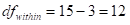
Within Degrees of freedom
, where K is the number of categories or groups, N is still the total N
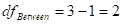
Between Degrees of freedom
We will also use degrees of freedom to locate the critical value on the F-table (see page A-29 for alpha .05 and A-30 for alpha .01). The numerator of the F-ratio is the between factor, so we will use the degrees of freedom between along the top of your table. The denominator of the F-ratio is the within subjects factor, so will use degrees of freedom within along the left margin of the table.
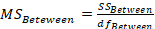
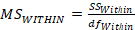
Mean Square
Now we divide each sums of squares by the respective mean square. Don’t let the formula’s intimidate you. All we are doing is matching up degrees of freedom with the Sums of squares to get the mean square (variance)
Within Mean Square
Between Mean Square
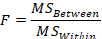
F-ratio
The final step is to divide our between by within variance to see if the effect (between) is large compared to the error (within).
Example
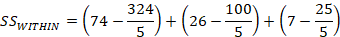
A therapist wants to examine the effectiveness of 3 therapy techniques on phobias. Subjects are randomly assigned to one of three treatment groups. Below are the rated fear of spiders after therapy. Test for a difference at α = .05
Table 1
| Therapy A | Therapy B | Therapy C |
| 5 | 3 | 1 |
| 2 | 3 | 0 |
| 5 | 0 | 1 |
| 4 | 2 | 2 |
| 2 | 2 | 1 |
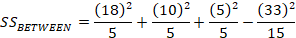
= 18
= 10
= 5
= 74
=26
= 7
STEP 1: State the null and alternative hypotheses.
H1 at least one mean differs
H0: m1 = m2 = m3
STEP 2: Set up the criteria for making a decision. That is, find the critical value.
You might do this step after Step 3 since that is where you compute the critical value.
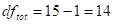
= 3-1 = 2
= 15-3 = 12
Fcritical = 3.88
STEP 3: Compute the appropriate test-statistic.
Although in this example I have given the summary values, for some problems you might have to compute the sum of x, and sum of squared x’s yourself.
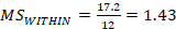
=


Note that anytime you compute two of the Sums of Squares you can derive the third one without computation because Between + Within = Total


Once we have computed all the values, very often we place them in a source table (below). Putting the values in a table like this one may make it easier to think about the statistic. Notice that once we get the Sums of Squares on the table, we will divide those values by the df in the next column. Once we get the two mean squares we divide those to get F as shown in Table 2.
Table 2
| Source | SS | Df | MS | F |
| Between or Group | 17.2 | 2 | 8.6 | 6 |
| Within or Error | 72 | 12 | 1.43 | |
| Total | 34.4 | 14 |
STEP 4: Evaluate the null hypothesis (based on your answers to the above steps).
Reject the null
STEP 5: Based on your evaluation of the null hypothesis, what is your conclusion?
There is at least one group that is different from at least one other group.