Lesson 4
Measures of Central Tendency
Outline
Measures of a distribution’s shape
-modality and skewness
-the normal distribution
Measures of central tendency
-mean, median, and mode
Skewness and Central Tendency
Measures of Shape
With frequency distribution you can an idea of a distribution’s shape. If we trace the outline of the edges of the frequency bars you can idea about the shape, as shown in Figure 1.
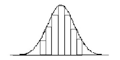
Figure 1
From this point on, I will draw these shapes to illustrate different point throughout the semester. Keep in mind what you are looking at is a line indicating the frequency or how many values in a distribution lie at a particular point on the scale: just like a histogram (see Figure 2).
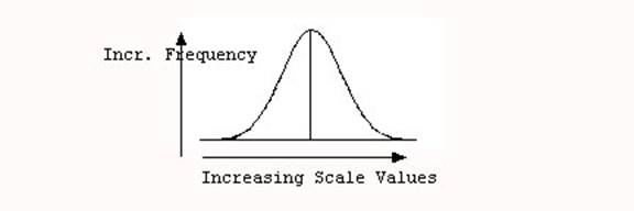
Figure 2
Modality – measures the number of major peaks in a distribution. A single major peak is unimodal, and is the most common modality. Two major peaks is a bi-modal distribution (see Figure 3). You could also have multi-modal distributions.
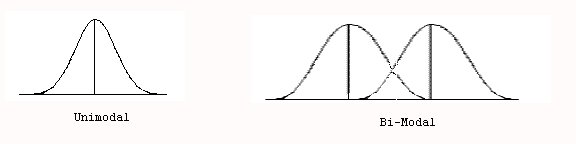
Figure 3
Skewness – measures the symmetry of a distribution. A symmetric distribution is most common and is not skewed. If the distribution is not symmetric, and one side does not reflect the other, then it is skewed. Skewness is indicated by the “tail” or trailing frequencies of the distribution. If the tail is to the right it is a positive skew. If the tail is to the left, then it is a negatively skewed distribution. For example, a positively skewed distribution would be: 1, 1, 2, 2, 2, 3, 3, 3, 9, 10. The outliers are on the high end of the scale. On the other hand, a negatively skewed distribution might be: 1, 2, 9, 9, 9, 10, 10, 10, 11, 11, 11. Here, and depicted in Figure 4, the outliers are on the low end of the scale.
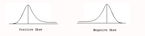
Figure 4
The normal distribution is one that is unimodal and symmetric. Most things we can measure in nature exhibit a normal distribution of values. Regression toward the mean is an idea that states values will tend to cluster around the mean with few values toward the trailing ends or “tails” of the distribution. As a result, most things we measure will tend to have a normal shape. Think about measures of height. There are very few people that are extremely tall or extremely short, but most tend to cluster around the average. With I.Q. scores, measures of weight, or most anything we can measure, the same pattern will repeat. Since most things we measure have more values close to the mean, we end up with mostly “normally” shaped distributions (see Figure 5).
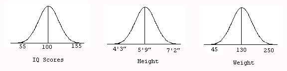
Figure 5
Measures of Central Tendency
Knowing where the center of a distribution is tells us a lot about a distribution. That’s because most of the scores in a distribution will tend to cluster about the center. Measures of central tendency give us a number that describes where the center lies (and most scores as well).
Mean – The mean, or average score, is the arithmetic center of the distribution. You can find the mean by adding all the scores () together and dividing by the number of values you added together (N), as shown in Table 1.
Table 1
| X |
| 1 |
| 2 |
| 3 |
| 4 |
| 5 |

N = 5
For the Population: =
= 3
For the Sample: =
= 3
Note that we calculate the mean the same way for both the sample and the population we symbolize them differently. Other statistics will differ in how they are computed for the sample versus the population.
Most students are familiar with these measures of central tendency, but there are several properties that may be new to you. 1) The first property of the mean is that it is the most reliable and most often used measure of central tendency. 2) The second property of the mean is that it need not be an actual score in the distribution. 3) The third property is that it is strongly influenced by outliers. 4) The fourth property is that the sum of the deviations about the mean must always equal zero.
The last two properties need further explanation. An outlier is an extreme score. It is a score that lies apart from most of the rest of the distribution. If there are several outliers in a distribution it will often result in skewed shape to the distribution. Outliers tend to pull central tendency measures with them. Thus a distribution of values 1, 2, 3, 4, 5 has an average of 3. Three does a good job of describing where most of the scores in this distribution lie. However, if there is an outlier, say by substituting 25 for the 5 in the above distribution, then the mean changes a great deal. The new distribution 1, 2, 3, 4, 25 has a mean of 7. Seven is not really close to most of the other values in the distribution. Thus, the mean is a poor measure of the center when we have outliers, or a skewed distribution.
A deviation is just a difference. A deviation from the mean is the difference between a score and the mean. So, when we say the sum of the deviations about the mean must always equal zero is just a way of saying that there are just as many differences between values above the mean and the center as there are differences between values below the mean and the center. Thus, for a simple distribution 1, 2, 3, 4, 5 the average is 3. Let’s use population symbols and say μ = 3. The deviations are the differences between the score and the mean, as shown in Table 2.
Table 2
| X | X-µ |
| 1 | 1-3 = -2 |
| 2 | 2-3 = -1 |
| 3 | 3-3 = 0 |
| 4 | 4-3 = 1 |
| 5 | 5- 3 = 2 |
μ = 3 = 0
Now if we add these deviations we will always get zero, no matter what original values we use. This concept will be important when we consider standard deviation because we will need to look at differences between values in our distribution and the mean.
Median – The median is the physical center of the distribution. It is the value in the middle when the values of the distribution are arranged sequentially. The distribution: 1, 1, 2, 2, 3, 4, 5, 5, 5, 6, 7 has a median value of 4 because there are five values above this point and five values below this point in the distribution:
1, 1, 2, 2, 3, 4, 5, 5, 5, 6, 7.
If you have an even set of numbers then there will be two values that are at the center, and you average these two values together in order to determine the median. For example, if we take out one of the numbers in the distribution so that we have
1, 1, 2, 2, 3, 4, 5, 5, 5, 6 then the two values in the center are 3 and 4
1, 1, 2, 2, 3, 4, 5, 5, 5, 6. The average of these two numbers is 3.5 and that is the median.
The median is resistant to outliers. That is, outliers will generally not affect the median and it will not be affected as much as the mean. It is possible the median might move slightly in the direction of the skew or outliers in the distribution.
Mode – The mode is the most frequent value in the distribution. It is simply the value that appears most often. For example in the distribution: 1, 1, 2, 3, 3, 3, 4, 4, 4, 4, 5, 6, 7 there is only one mode (4). But, in the distribution: 1, 1, 2, 3, 3, 3, 3, 4, 4, 4, 4, 5, 6 there are two modes (3 and 4). If there is only one of each value then there is no mode.
The mode is not affected by outliers. Since it is only determined by one point on the scale, other values will have no effect.
Skewness and Central Tendency
We have already discussed how each measure is affected by outliers or skewed distribution. Let’s consider this information further. In a positively skewed distribution the outliers will be pulling the mean down the scale a great deal. The median might be slightly lower due to the outlier, but the mode will be unaffected. Thus, with a negatively skewed distribution the mean is numerically lower than the median or mode, as shown in Figure 6.
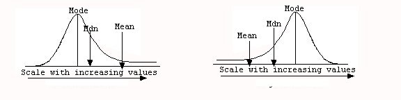
Figure 6
The opposite is true for positively skewed distributions. Here the outliers are on the high end of the scale and will pull the mean in that direction a great deal. The median might be slightly affected as well, but not the mode. Thus, with a positively skewed distribution the mean is numerically higher than the median or the mode.